Introduction
Most financial models assume returns follow a clean bell curve — symmetric, predictable, and well-behaved. Real market data refuses to cooperate.
Asset prices trend and drift in ways that violate basic regression assumptions. Returns cluster into volatile and calm regimes. Extreme losses appear far more often than any normal distribution would predict. And the sequence in which observations occur carries information that cross-sectional analysis simply ignores.
These aren't minor technical footnotes. They determine which models are valid, how risk gets measured, and whether a forecast is trustworthy or spurious.
This article covers the statistical foundations analysts need to work with financial time series properly: distribution properties, stationarity, autocorrelation, volatility behavior, and the model selection trade-offs each concept drives.
Key Takeaways
- Financial returns consistently show fat tails and frequent non-normality — extreme losses occur more often than standard models predict
- Asset prices are almost always non-stationary; log returns generally are, a distinction that directly shapes which models apply
- Autocorrelation in squared returns (not raw returns) is the statistical signature of volatility clustering
- Statistical significance ≠ economic significance with large datasets — evaluating both independently is essential before acting on findings
- Choose models (ARIMA, GARCH, etc.) based on the data's actual statistical properties — not analytical convenience
What Makes Financial Time Series Unique
A financial time series is a sequence of observations recorded at regular intervals — daily RevPAR, monthly occupancy rates, equity returns, interest rates — where the order of observations carries information. That last clause is what separates time series from ordinary cross-sectional data, and it changes everything about how the data must be handled.
In cross-sectional data, you can shuffle the rows without losing anything meaningful. In time series, observation order is the data. Past values may predict future values, volatility may cluster across adjacent periods, and errors are rarely independent.
This breaks the standard regression assumption of independently and identically distributed (i.i.d.) errors. As Cont's cross-market synthesis documents, financial returns show heavy tails, volatility clustering, and persistent autocorrelation in absolute returns — none of which are consistent with i.i.d. behavior.
Prices vs. Returns
In practice, analysts work with returns rather than raw prices. Three properties make returns preferable:
- Sum of one-period log returns equals the log return over the full interval (time-additivity)
- Returns don't trend or drift the way prices do, making them closer to stationary
- Returns are closer to symmetric with finite variance under most market conditions
The log return formula: r_t = ln(P_t) - ln(P_{t-1})
Deterministic vs. Stochastic Components
Most real financial series contain both:
- Deterministic components: trends (long-run directional drift), seasonality (Q4 hotel demand spikes, summer leisure travel peaks), and business cycles (macro expansions and contractions)
- Stochastic components: random shocks from geopolitical events, pandemics, sudden credit dislocations
No model eliminates random shocks entirely. What disciplined forecasting does is decompose these components and model each on its own terms, improving decision-making even when certainty isn't available.
The Distribution Problem: Fat Tails, Skewness, and Kurtosis
The single most common mistake in financial analysis is assuming returns follow a normal distribution. A normal distribution implies symmetric outcomes and vanishingly rare extreme events. Financial returns deliver neither.
Skewness: Why Markets Fall Faster Than They Rise
Skewness measures distributional asymmetry. Equity returns frequently show negative skewness — large negative moves occur more often than equivalent positive moves. Markets tend to fall sharply and recover gradually.
This is a measurable statistical property with direct portfolio construction implications. Strategies that look attractive on mean-return metrics can carry asymmetric downside exposure that summary statistics hide.
Skewness direction is asset-class dependent. While negative skewness is well-documented in equities, commercial real estate and commodity futures show varied skew signs across samples and periods. The defensible cross-asset claim: fat tails and non-normality are widespread; skewness direction must be tested per asset and sample.
Kurtosis and Fat Tails: When "Rare" Events Keep Happening
Excess kurtosis measures how much probability mass sits in the tails beyond what a normal distribution predicts. Financial returns almost universally display high positive excess kurtosis — fat tails.
An analyst who assumes normality when modeling a fat-tailed distribution will systematically underestimate the frequency of extreme losses. That underestimation is the mechanism behind so-called "multi-sigma events" appearing in markets far more often than theory predicts.
Two standard diagnostic tools:
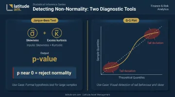
- Jarque-Bera test: Formally tests normality using both skewness and kurtosis. For most financial return series, the JB test rejects normality with near-zero p-values — though rejection doesn't isolate whether skewness, kurtosis, or both are responsible.
- Q-Q plots: Plot empirical quantiles against theoretical normal quantiles. Financial return data produces a characteristic S-shape at both ends, indicating more extreme observations than a normal distribution would generate.
Stationarity and How to Test for It
Why Stationarity Is Non-Negotiable
A time series is stationary when its mean, variance, and autocorrelation structure remain constant over time. Most forecasting models — ARIMA, GARCH, regression — require stationarity. Applying them to non-stationary data produces spurious correlations and unreliable results that can look significant while being entirely meaningless.
The critical distinction: asset prices are almost always non-stationary (they trend and drift); log returns are typically stationary. This is the core reason analysts transform prices into returns before modeling.
The Augmented Dickey-Fuller Test
The ADF test is the standard method for testing stationarity. Its mechanics:
- Null hypothesis: Unit root present = non-stationary
- p < 0.05: Reject the null; series is stationary
- p ≥ 0.05: Fail to reject; treat series as non-stationary
Price series typically fail to reject the unit-root null. Return series typically reject it. Structural breaks — like the 2020 COVID shock that sent U.S. hotel RevPAR down 47.5% to $45.48 — can reduce ADF test power, so a failed rejection around crisis periods isn't always conclusive.
The Practical Sequence
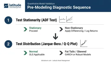
The recommended diagnostic order:
- Test stationarity (ADF) — determines whether transformation (differencing, log returns) is required before any model is fit. Skipping this step risks building on a drifting baseline.
- Test distributional properties (Jarque-Bera, Q-Q plot) — identifies fat tails, skewness, or other non-normality that rules out standard OLS assumptions and points toward GARCH-family or robust alternatives.
Run both tests before committing to a model. Stationarity tells you whether to transform the data; distributional shape tells you which model class can handle what remains.
Autocorrelation, Volatility Clustering, and the Leverage Effect
Two Types of Autocorrelation
Autocorrelation measures whether today's value depends on past values. In financial time series, two distinct types matter:
- Autocorrelation in raw returns: Tests whether price direction is predictable — directly relevant to market efficiency debates
- Autocorrelation in squared returns: Tests whether the magnitude of moves clusters — relevant to risk management and volatility modeling
Raw return autocorrelation is often statistically insignificant beyond very short horizons. That doesn't mean returns are independent — nonlinear dependence can persist even when linear autocorrelation is absent.
Volatility Clustering
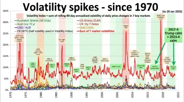
Volatility clustering is one of the most robustly documented properties of financial returns: large moves tend to follow large moves; calm periods tend to follow calm periods. Rolling volatility charts consistently show elevated volatility clustering around market crises before subsiding — 2008, 2020, and 2022 all followed this pattern.
For asset managers, this has a direct practical implication: if volatility today is elevated, tomorrow's risk exposure is likely elevated too. Risk is not constant across time. Position sizing and hedge ratios that assume static volatility will be wrong precisely when it matters most.
The statistical signature: a slowly decaying, positive autocorrelation function (ACF) in squared or absolute returns. This is the standard diagnostic for ARCH effects.
Statistical vs. Economic Significance
With large datasets — thousands of daily return observations — confidence intervals shrink dramatically. Trivially small autocorrelations become statistically significant. A correlation that passes a statistical threshold may still be economically meaningless after accounting for transaction costs, execution slippage, and signal decay.
The dual-filter approach requires a correlation to clear both bars before it deserves further investigation:
- Statistical threshold: passes p-value or confidence-interval cutoff
- Economic threshold: large enough to matter in practice after costs
A concrete example: suppose a daily autocorrelation of 0.03 is detected with p < 0.01 in a 5,000-observation dataset. Statistically significant. But a 3% directional signal, after bid-ask spread and execution costs, likely produces no tradeable edge. Economic significance requires effect size evaluation, not just p-values.
The Leverage Effect
The leverage effect describes an asymmetry in how return shocks affect future volatility: negative shocks increase future volatility more than positive shocks of equal magnitude.
This has two concrete implications:
- Options pricing: The asymmetry manifests as a volatility skew — out-of-the-money puts command higher implied volatility than equivalent calls
- Risk management: Downside moves should trigger proportionally larger increases in hedge ratios than equivalent upside moves; symmetric GARCH specifications may understate this risk
Key Statistical Models for Financial Time Series
ARIMA: Capturing Trend and Autocorrelation
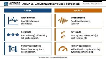
ARIMA (Autoregressive Integrated Moving Average) is the standard framework for modeling stationary time series with autocorrelation in the conditional mean. Its three components:
| Component | Role | Parameter |
|---|---|---|
| Autoregressive (AR) | Uses past values to predict future values | p lags |
| Integration (I) | Differences the series to achieve stationarity | d differences |
| Moving Average (MA) | Uses past forecast errors | q lags |
Primary use cases: short-term return or economic indicator forecasting, decomposing series with trend and autocorrelation. ACF and PACF plots guide lag selection — slowly decaying ACF suggests AR structure; cut-off patterns suggest MA terms.
GARCH: Modeling Volatility Dynamics
GARCH (Generalized Autoregressive Conditional Heteroskedasticity) models not the level of a series but its conditional variance. The GARCH(1,1) specification:
h_{t+1} = ω + α·ε_t² + β·h_t
Today's forecast variance depends on yesterday's squared innovation (α) and yesterday's conditional variance (β). The key constraint for covariance stationarity: α + β < 1.
GARCH captures what ARIMA cannot — the memory in volatility itself. Applications:
- Value-at-Risk (VaR) calculations: Dynamic risk estimates that adjust to current market conditions
- Options pricing: Duan (1995) formalizes how conditional GARCH volatility enters option valuation
- Portfolio construction: Time-varying risk estimates for dynamic position sizing
Two diagnostic tools round out model validation. The Ljung-Box test jointly tests whether a group of autocorrelations is zero; applied to model residuals, rejection indicates remaining serial structure the fitted model hasn't captured. For series with strong seasonal patterns (hotel revenue metrics being a clear example), decomposition methods separating trend, seasonality, and residual components are essential before any ARIMA or GARCH specification is attempted.
Applying Time Series Insights to Investment Decisions
The statistical properties covered here aren't abstractions — they directly affect how investment decisions get made.
Three critical applications:
- Risk management: Fat tails mean constant-volatility models will underestimate drawdown probability during stress periods. A model calibrated to recent calm data will produce inadequate risk estimates precisely when a market dislocation strikes.
- Asset selection and timing: Volatility clustering means risk levels are time-varying. Entry timing and position sizing should adjust based on current volatility regime, not historical averages.
- Performance forecasting: Stationarity and autocorrelation structure determine which forecasting models are valid for a given data series. Fitting a stationary model to a non-stationary series isn't just suboptimal — it produces results that are statistically meaningless.
Hospitality operating metrics are themselves financial time series: RevPAR trends, occupancy rates, ADR trajectories, and net operating income all carry seasonality (Q4 leisure demand spikes, summer slowdowns), cyclical patterns tied to GDP, and event-driven discontinuities.
The 2020 U.S. hotel market recorded a 47.5% RevPAR decline in a single year. That observation should not be modeled as ordinary seasonal variation — it is a structural break requiring separate treatment.
Applying the same statistical rigor used in equity analysis to hotel performance data enables more accurate underwriting and scenario modeling. At Latitude Asset Management, Javier Revelo, CFA — whose career spans institutional portfolio risk management and hospitality analytics — leads financial analysis across acquisitions, portfolio strategy, and performance evaluation throughout the Americas. That discipline means treating performance metrics as time-varying inputs, not static averages.
No model replaces domain expertise, but understanding the true statistical behavior of financial data prevents systematic errors. Using constant-volatility assumptions during high-turbulence periods — or treating statistically significant autocorrelations as economically actionable without a second filter — compounds across every subsequent decision. The strongest investment frameworks combine quantitative rigor with the operational and market-specific knowledge to interpret what the data is actually saying.
Frequently Asked Questions
What is a financial time series and how is it different from regular data?
A financial time series is a sequence of observations where the order carries information: past values may predict future ones, and errors are rarely independent. Unlike cross-sectional data, where you can shuffle rows without losing anything, the sequence itself is part of the data structure, which makes standard i.i.d. statistical assumptions routinely inappropriate.
Why do financial returns have fat tails and what does that mean for risk?
Fat tails reflect the empirical tendency for extreme price moves to occur far more often than a normal distribution predicts. For risk management, the implication is direct: models assuming normality will consistently underestimate the probability of large losses, leaving portfolios underhedged precisely during market dislocations.
What is stationarity and why does it matter for time series modeling?
Stationarity means the statistical properties of a series — mean, variance, autocorrelation structure — remain constant over time. Most forecasting models require it. Asset prices are typically non-stationary (they trend); log returns generally are, which is why analysts transform prices before modeling.
What is volatility clustering and how is it detected?
Volatility clustering is the documented tendency for large market moves to follow large moves, and calm periods to follow calm periods. It's detectable through the ACF of squared returns: a slowly decaying, positive pattern confirms clustering. Rolling volatility charts make it visible too, showing elevated variance concentrated around historical market crises.
What is the difference between ARIMA and GARCH models?
ARIMA models the level of a time series, using past values and past errors to forecast future values. GARCH models the variance — specifically how conditional volatility evolves over time based on past squared innovations and past variance estimates. ARIMA addresses serial dependence in the mean; GARCH addresses it in risk.
How do analysts distinguish statistically significant autocorrelation from noise in large datasets?
With large datasets, even trivially small correlations become statistically significant. Analysts apply a dual filter: the correlation must clear a statistical threshold (distinguishable from noise) and an economic one (meaningful after transaction costs). Only signals that pass both are treated as actionable.